Design report

A user can download all characteristics of a design with the functionality available at the Design detail page:

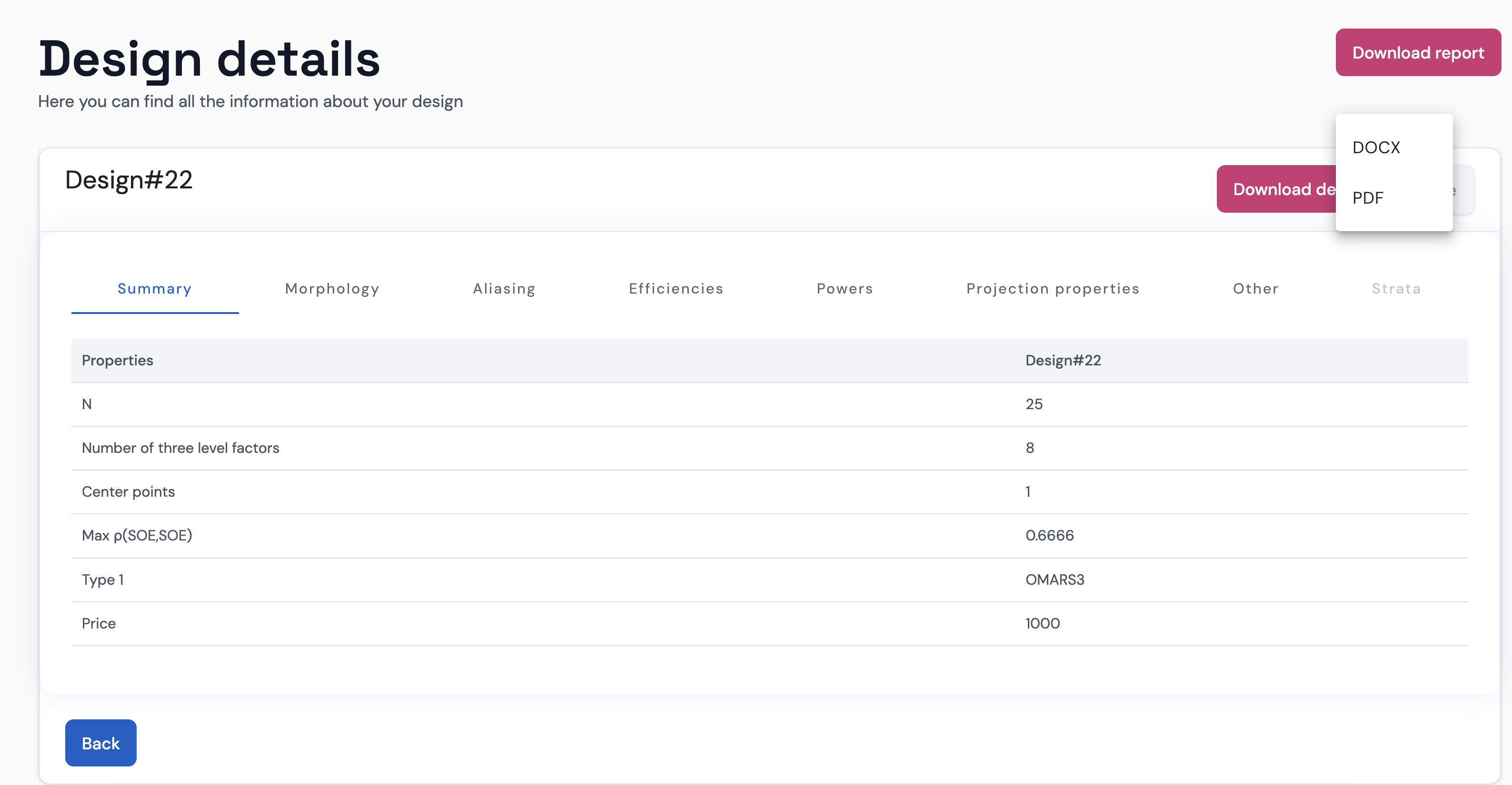
The characterization in PDF format is available for all designs, while the characterization in Word format is only available for purchased designs.

The report is structured in 9 sections:

1. Summary
2. Morphology
3. Aliasing
4. Efficiencies
5. Fraction of design space plots
6. Powers for effect types and deifferent estimable models
7. Projection properties
8. Model effects related characteristics
9. Powers for model effects and different estimable models

We now explain each section in detail.

1. Summary

• Number of runs: number of tests of the experimental design.
• 3-level factors: number of factors that are studied at three levels, which correspond to the minimum, average and maximum values of a given continuous range. These factors allow the estimation of main and quadratic effects and they are used to model quantitative factors.
• 2-level factors: number of factors that are studied at two levels. These factors can be used to model either quantitative or categorical factors with two levels. If a 2-level factor is quantitative, then the two-levels correspond to the minimum and maximum values of a given continuous range. If the 2-level factor is categorical, then the two levels indicates the two categories that the factor can take. All the characterizations of the designs consider the 2-level factors as categorical.
• Center points: number of tests of an experimental design where all 3-level factors are set to their average value.
• Maximum 4th order correlation: maximum value of the absolute correlation between two second-order terms (this is, between two-factor interaction effects and/or quadratic effects).
• Number of blocks: number of groups of runs that the design is partitioned in. In our catalog, the blocking factor is orthogonal to all main effects.
• Block size: number of runs per block. In our catalog, all blocks have the same size.

2. Morphology

• Degrees of freedom for pure error: the responses of the replicated runs of a design can be used to estimate the pure error independently from the model. This enables a lack-of-fit test while modeling the data. The Degrees of freedom for pure error takes all replicates into account (center runs and any other replicated runs).
• Number of replicates: indicates how many different runs are replicated in the design. The higher the value, the higher the coverage of the design space when calculating the pure error.
• Mirror: equals true if the design has a foldover structure, this is, for every run in the design, the run result of switching the low and high values in all the factor levels is also present in the design.
• Uniform precision in the main effects: indicates if all columns of the 3-level factors have the same number of entries equal to the factor average level. It indicates that the power to detect a single main and/or quadratic effects is the same for all factors.
• Uniform precision in the interaction effects: indicates if all columns of the two-factor interactions in the model matrix have the same number of entries equal to zero. It indicates that the power to detect a single interaction effect is always the same.
• Intrablock correlation coefficient: when a design has a random blocking factor, there are two sources of variation: $\sigma^2_{\varepsilon}$ which quantifies the residual error variance, and $\sigma^2_{\gamma}$ is the block variance. The ratio between these two variances is denoted as $\eta=\sigma^2_{\gamma}/\sigma^2_{\varepsilon}$. The intrablock correlation coefficient equals $\frac{\eta}{\eta+1}$. If there are no blocks, then both $\eta$ and the intrablock correlation coefficient equal zero and the introblock correlation is not reported. If the blocks are treated as a fixed effect, the intrablock correlation coefficient equals $1$. When the blocks are treated as a random effect, the intrablock correlation coefficient lies between $0$ and $1$.

3. Aliasing

• Balanced main effects: indicates if the number of times any factor is set to its lower level equals the number of times the same factor is set to its upper level.
• Average 2nd order correlation: average value of the absolute correlation between the main effects of two factors.
• Maximum 2nd order correlation: maximum value of the absolute correlation between the main effects of two factors.
• Average 3rd order correlation: average value of the absolute correlation between the main effect of a factor and a second-order effect.
• Maximum 3rd order correlation: maximum value of the absolute correlation between the main effect of a factor and a second-order effect.
• Average 4th order correlation: average value of the absolute correlation between two second-order effects.
• Maximum 4th order correlation: maximum value of the absolute correlation between two second-order effects.
• OMARS: equals true if the design is an Orthogonal Minimally Aliased Response Surface Design, this is, when the main effects are balanced, and the maximum 2nd and 3rd order correlation equals $0$.
• Maximum eta correlation between the block effect and a main effect: maximum value of the correlation¹ between the block effect and a main effect.
• Maximum eta correlation between the block effect and an interaction effect: maximum value of the correlation¹ between the block effect and an interaction effect.
• Maximum eta correlation between the block effect and a quadratic effect: maximum value of the correlation¹ between the block effect and a quadratic effect.
• Maximum eta correlation between the block effect and a second-order effect: maximum value of the correlation¹ between the block effect and a second-order effect.

4. Efficiencies

In this section we present the most common efficiencies for the statistical models that are estimable. The models are of the next four different types:

• ME model: this includes all the main effects of the original factors
• ME + IE model: this includes all the main effects and two-factor interactions
• ME + SOE model: this includes all the main effects and second order effects (two-factor interactions and quadratic effects).
• ME + QE model: this includes all the main effects and the quadratic effects.

The characteristics reported are the D-, A- and G-efficiency and the average prediction variance.

5. Fraction of design space plot

The fraction of design space plot indicates the distribution of the prediction variance across the design space. This plot is obtained by calculating the prediction variance of random points within the design space and ordering them. In the horizontal axis one can find the value of the prediction variance, while on the vertical axis we indicate the fraction of design space. For example, if we draw an horizontal line from the point located at the vertical coordinate $0.5$and we intersect it with the curve, we obtain a prediction variance such that the %50%$ of the design space has a prediction variance equal or lower to it.

We provide a plot for every estimable model (ME, ME+IE, ME+SOE and ME+QE models).

6. Powers for effect types and different statistic models

In this section there are three tables, one for each of three significance levels $\alpha \in {0.01, 0.05, 0.1}$. Each table contains the powers to detect model effects for five different values of the signal-to-noise-ratio (SNR). The other headers in the table are:

• Model: underlying model considered in the power calculation
• Effects: effect type considered, which can be main, interaction of quadratic effect.

Each entry in the table is the minimum power to detect the effect type, with the underlying model at the SNR and alpha indicated.

7. Projection properties

This section consists of two tables. The first table offers details on the estimation quality of second-order models based on subsets of the factors. For any subset, these models include an intercept, all the main effects, all the two-factor interactions, and all the quadratic effects of the numerical three-level factors in the subset. The second table offers details on the estimation quality of a model with main and interaction effects based on subsets of the factors. For any subset, these models include an intercept, all the main effects, and all the two-factor interactions.

Both tables have the same columns:

• f3: number of 3-level factors considered
• f2: number of 2-level factors considered
• total, OK, %: total number of projection models, number of estimable models that are estimable, and the percentage
• D-efficiency: average D-efficiency for all the estimable projection models
• A-efficiency: average A-efficiency for all the estimable projection models
• G-efficiency: average G-efficiency for all the estimable projection models
• Prediction variance: average average prediction variance for all the estimable projection models

The columns labeled as f3 and f2 give information on how many 3- and 2-level factors are considered in the projection models. The columns total, OK, % indicate the estimability of those models. Finally, the rest of the columns indicate how well these models can be estimated and how precise the estimation is.

8. Model effects related characteristics

We provide here information on the relative standard error (REE), the fracional increase in confidence interval length (FICIL), and the variance inflation factors (VIF) for the individual effects in every estimable model.

9. Powers for model effects and different estimable models.

Powers to detect individual effects in every estimable models for different significance levels and signal-to-noise ratios.

Page last modified on 26 February 2025