Define your experiment

In this tab, you specify the number of factors in your experiment, the type of these factors and the target model that you want to fit.

Experimental factors

Enter the number of three-level factors and the number of two-level factors involved in your experiment using the input boxes.

You can include two different kinds of experimental factors: two-level categorical or continuous factors, and three-level continuous factors. The experimental factors are also called independent variables, or controllable factors. For each type mentioned, it is important to know when to use them to model the effects of the experimental factors:

• Two-level factors are used to model experimental factors that can take two different values.

  • Two-level factors can be used with both continuous and categorical factors. One the one hand, when the factor is quantitative, the first level corresponds to the lower level and the second level to the upper level of the interval wherein the factor varies.

  • Examples: a categorical factor that indicates if the experiment is performed by either machine A or machine B, or a continuous factor that indicates the low and high value of temperature investigated at two levels only.

  • Technical considerations (click to unfold)

    • The two different values of two-level factors are coded as $-1$ and $1$.
    • It is not possible to estimate the quadratic effect of a continuous experimental variable modeled as a two-level factor.
    • For calculation of prediction variances, two-level factors are taken as categorical.

• Three-level factors are used to model quantitative experimental factors.

  • The factors are assumed to vary within a closed continuous interval and three values are considered when planning the experimental design: design: the lowest and highest value of the interval and the value in between these values.

  • Example: a factor that indicates the temperature of an experiment which can take values within a given range.

  • Technical considerations (click to unfold)

    • The three values are coded as:
      • Low value: $-1$
      • Medium value: $0$
      • High value: $1$
    • Three-level factors allow the user to study quadratic effects in addition to the main effects and two-factor interaction effects.

The software database contains hundreds of thousands of experimental designs that contain only three-level factors. The most important family of experimental designs are OMARS designs ¹. For these designs, all main effects can be independently estimated from each other and from any other second-order effect (2-factor interaction effects and quadratic effects). Standard designs such as Definitive Screening Designs, Central Composite Designs and Box-Behnken designs are examples of OMARS designs.

When you combine two- and three-level factors, you will end up with what is known as a mixed level design. To the best of our knowledge, our database is the only one with OMARS mixed level designs². For these designs, all the three level and two level factors have all main effects orthogonal to each other and to all second order effects.

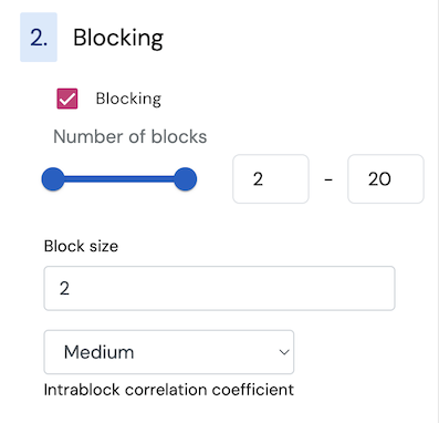
Blocking

Very often there are blocking factors that can potentially influence the response. Check this box if you would like to use an additional blocking factor with your design.

Blocking is very common in experiments and is often implemented when groups of experimental runs are performed under different or non-homogenous experimental conditions. For example, a number of experiments could be run during the course of multiple days. In such a case, the ‘day’ in which the runs are performed could be treated as a blocking factor. This can be done by introducing a blocking factor in the design. When the blocking option is checked, the software always produces designs where the blocking factor is orthogonal to all main effects of the original factors and hence the final design selected will allow the user to study the main effects from the original factors independent from the blocking factor.

The controls to include a blocking factor in an experimental designs are:

• Number of blocks and block size.

  • Most often the number of runs that can be performed in a single block (group) of experimentation is known in advance. For example, the blocking factor can be a day and the block size is determined by how many tests can be carried out in one day.
  • Once the block size is fixed, you can use the range slider to set the number of blocks. This will allow you to compare experimental plans with different number of blocks with each other, and assess what the trade-off between the run size and the quality of the design is.
  • The number of runs of the experimental design equals the block size multiplied by the number of blocks.
  • Example: in a cake baking experiment, if it can be expected that different baking ovens used will produce non-homogenous baking conditions, then in such a case, the oven used can be treated as a blocking variable. In such a case, the number of blocks would be set as the number of different ovens used during the experiments.

• Intrablock correlation coefficient is used to indicate how different the blocks are from each other. It equals the ratio between the variance between the blocks and the error variance.

  • A value of EXTREME corresponds to the situation when the blocks are expected to be very different from each other and they will be modeled as a fixed block effect.
  • The values LOW, MEDIUM and HIGH correspond to a coefficient equal to 0.1, 1 and 10, respectively. Any of these three options indicate that the block effect will be treated as a random block effect.
  • The default value in the software is MEDIUM.
  • Technical considerations (click to unfold)

    • To define the nature of the block, we need to consider two sources of variation. On the one hand, two observations coming from runs within the same block are expected to differ from each other according to the residual error variance. On the other hand, two observations coming from different blocks are, additionally, expected to differ from each other according to the sum of the residual error variance and the variance between blocks. The ratio between the variance between blocks and the error variance is known as the intrablock correlation coefficient.
    • As mentioned earlier, the blocking factor can be treated as a fixed effect or a random effect. It is sensible to set the blocking factor as a fixed effect if the groups of runs in each individual block is expected to produce responses that are drastically different than the runs in another block. Modeling the blocking factor as a fixed effect, uses more degrees of freedom for estimation since each group or block is treated as a separate effect. However, if the runs in different blocks are considered to be only marginally different, then it is recommended to treat the blocking factor as a random effect which frees up a few degrees of freedom to estimate other effects involving the original factors which are often more important.

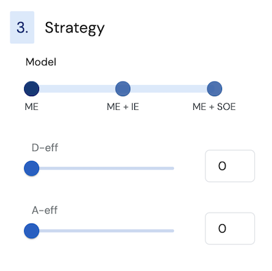
Strategy: model of interest and efficiencies

This important section of the controls allows the user to set the target statistical model, which indicates how many terms the linear model will consist of. After setting the model of interest with the slider, the user will be able to set a minimal value for both the D- and A-efficiency.

Below you can find more detailed information on how these controls work and the statistical theory behind them.

• The slider has three different fixed positions:

  • ME model: this includes all the main effects of the original factors
  • ME + IE model: this includes all the main effects and two-factor interactions
  • ME + SOE model: this includes all the main effects and second order effects (two-factor interactions and quadratic effects).
  • Note that the values are nested, which is indicated by the coloring of the slider bar which starts from the left side. For example, when a ME+IE model is selected, the slider is colored including also a ME model, which indicates that a ME model is also estimable.
  • Technical considerations (click to unfold)

    Consider an experiment with $m=m_1+m_2$ factors, with $m_1$ 3-level factors and $m_2$ 2-level factors. The designs in our catalog allow the estimation of a linear model that relates the factors and a response. The choice of the model needs to be done before selecting a design, as, for example, not all designs allow fitting all second-order effects.

    A ME model is given by the following equation:

    $ y = \beta_0 + \sum_{i=1}^{m} \beta_i x_i + \varepsilon $,

    where $y$ is the response, $\beta_0$ corresponds to the intercept, $\beta_i$ corresponds to the main effect of the $i$th factor, $x_i$ is the $i$th factor level, and $\varepsilon$ is the random error which is assumed to follow a normal distribution.

    A ME + IE model is given by the following equation:

    $ y = \beta_0 + \sum_{i=1}^{m} \beta_i x_i + \sum_{i=1}^{m-1} \sum_{j=i+1}^{m} \beta_{ij} x_i x_j + \varepsilon $,

    where $\beta_{ij}$ is the two-factor interaction effect between the $i$th and the $j$th factors.

    A ME + SOE model is given by the following equation:

    $ y = \beta_0 + \sum_{i=1}^{m} \beta_i x_i + \sum_{i=1}^{m-1} \sum_{j=i+1}^{m} \beta_{ij} x_i x_j + \sum_{i=1}^{m_1} \beta_{ii} x_i^2 + \varepsilon $,

    where $\beta_{ii}$ is the quadratic effect of the $i$th factor.

• The two sliders below allow the user to set a minimum limit on the D and A efficiencies for the design for the chosen model of interest.

  • This model will include the blocking factor if selected.
  • The next two sliders are used to set a lower limit on the D and A efficiencies for the model chosen. The slider ranges from 0 to 100%.
  • Technical considerations (click to unfold)

    The D and A-efficiencies are calculated as follows:

    $\text{D-efficiency} = \frac{\mathbf{{|X’X|}^{1/p}}}{N}$, and

    $\textit{A-efficiency} = \frac{p}{N \times tr\mathbf{{(X’X)}^{-1}}}$, where

    $\mathbf{X}$ is model matrix, $p$ is the number of effects of the statistical model (which equals the number of columns of the model matrix), and $N$ is the number of runs.

    When the design is organized in blocks, the calculations are different.

    • When blocking factor is treated as a fixed effect:

      $\text{D-efficiency} = \frac{\mathbf{{|[XZ]'[XZ]|}^{1/p}}}{N}$

      $\textit{A-efficiency} = \frac{p}{N \times tr\mathbf{{([XZ]'[XZ])}^{-1}}}$

      where $\mathbf{X}$ is the model matrix selected (ME, ME+IE, or ME+SOE) excluding the intercept, $\mathbf{Z}$ is the dummy coded matrix for the blocking factor, $\mathbf{[XZ]}$ is the concatenated full model matrix , $p$ is the total number of effects and $N$ is the number of runs.

    • When blocking factor is treated as a random effect:

      $\textit{D-efficiency} = \frac{\mathbf{{|X’V^{-1}X|}^{1/p}}}{N}$

      $\textit{A-efficiency} = \frac{p}{N \times tr\mathbf{{(X’V^{-1}X)}^{-1}}}$

      where $\mathbf{X}$ is the model matrix selected (ME, ME+IE, or ME+SOE) including the intercept, $\mathbf{V}$ is the variance-covariance matrix of all responses, p is the total number of effects and N is the number of runs. Here, $\mathbf{V}$ is adapted based on the intrablock correlation setting.

    It is important to note that the efficiency values will generally be low for three-level or mixed-level designs. This is because the efficiency is calculated in comparison to a theoretical optimal for a two level design.

    For a more thorough understanding of the concept of blocking, refer to Chapter 7 and 8 of Optimal design of experiments by Peter Goos, Bradley Jones [^gj].