Efficiencies
This tab displays the efficiencies for the models that are estimable.
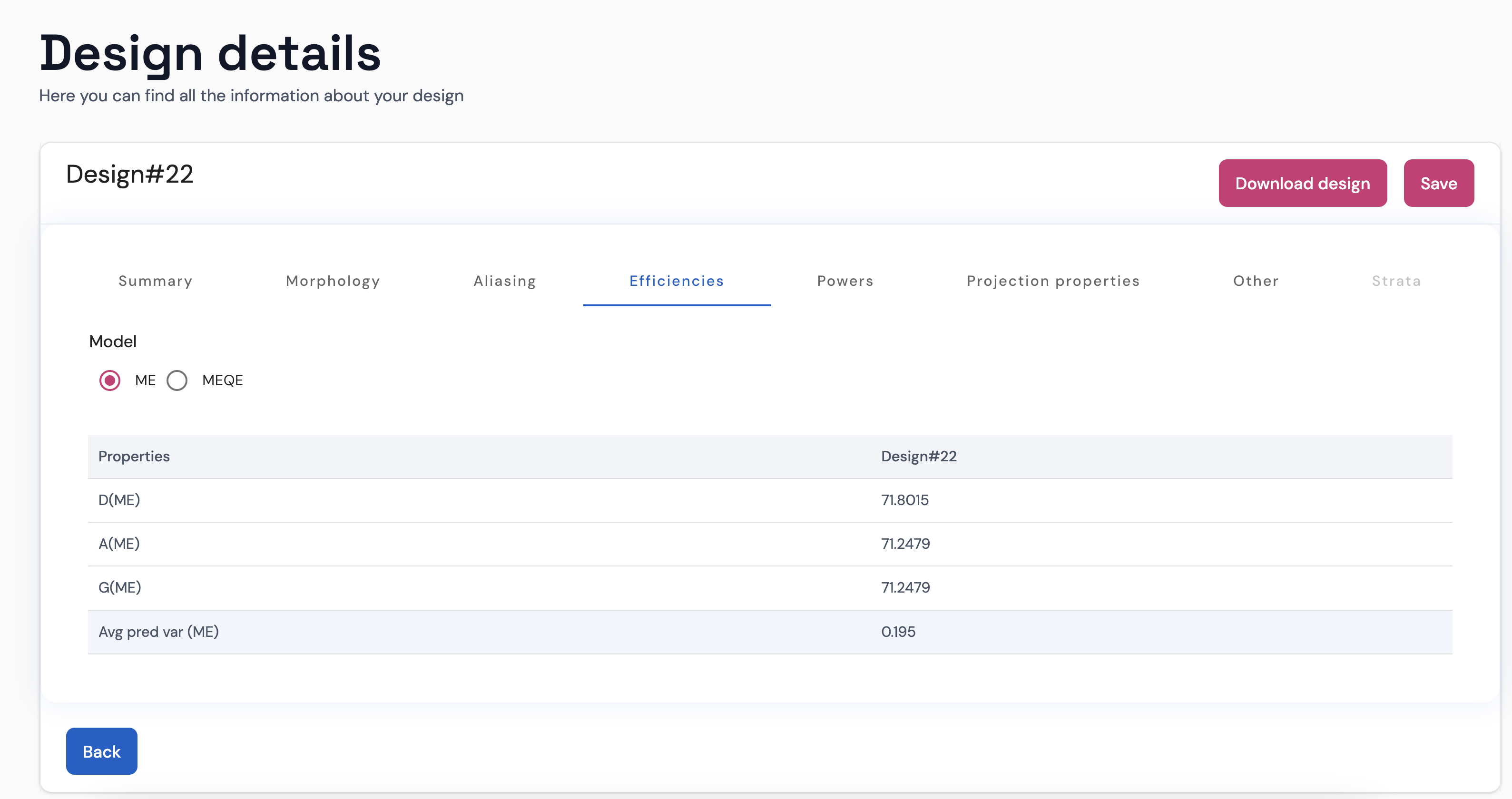
As in the previous tab, when you place the pointer of your mouse over the text on the Properties column, you will get an explanation. You can change the model using the radio buttons on top.
The D-, A-, G- and I-efficiency are standard attributes of an experimental design which inform us about how well the model effects are estimated and how precise the predictions will be. All efficiencies are, in one way or another, based on the Fisher information matrix.
Design matrix and model matrix
The design matrix, denoted as $\mathbf{D}$, has $n$ rows (one per test), and $m$ columns (one per factor). Schematically, it is represented as $\mathbf{D} = \begin{pmatrix} d_{11} & d_{12} & \cdots & d_{1m} \\ d_{21} & d_{22} & \cdots & d_{2m} \\ \vdots & \vdots & \cdots & \vdots \\ d_{n1} & d_{n2} & \cdots & d_{nm} \end{pmatrix}$, where an entry $d_{ij}$ indicates the level of the $j$-th factor at the $i$-th run.
The expansion vector function, denoted as $\mathbf{f}(\mathbf{d})$ takes a vector of factor settings (this is, a row of $\mathbf{D}$), and expands that vector to its correponding model terms, which can include intercept, main effects, two-factor interaction effects, quadratic effects, etc.
The model matrix, denoted as $\mathbf{X}$, has $n$ rows (one per test), and $p$ columns (one per effect). It is built by applying the expansion vector function to each row of the design matrix.
D-efficiency and A-efficiency
Notation:
- D-efficiency for a specific model: D(model)
- A-efficiency for a specific model: A(Model)
Both measure how precisely the effects in a model can be estimated.
The inverse of the information matrix, $(\mathbf{X}^T\mathbf{X})^{-1}$, indicates how well the model effects can be estimated. In an orthogonal design, where the model effects can be estimated independently from each other, both the information matrix and its inverse are diagonal matrices.
For example, the diagonal entries quantify the estimation error of each one of the model effects, and its determinant gives an overall measure on how good all model effects can be estimated compared to an orthogonal design.
The D-efficiency is a number that lies between $0$ and $100$ and gives us information on the confidence ellipsoid of the estimation error of the model effects. The lower this value, the better. It is calculated from the determinant of the information matrix as follows: $D-efficiency = 100 \cdot\frac{|\mathbf{X}^T\mathbf{X}|}{n}^{1/p}$, where $|\cdot|$ denotes the determinant of a matrix, $p$ is the number of effects in the model and $n$ is the number of runs. The D-efficiency takes into account the correlation between the estimates of the model effects.
The A-efficiency is a number that lies between $0$ and $100$ and, similarly to the D-efficiency, indicates how well the model effects can be estimated overall. It is calculated using the trace of the information matrix as follows: $A-efficiency = 100 \cdot \frac{p}{n \cdot tr((\mathbf{X}^T\mathbf{X})^{-1})}$, where $tr(\cdot)$ is a matrix operator result of the sum of the diagonal entries of the matrix (matrix trace).
G-efficiency and average prediction variance
Notation:
- G-efficiency for a specific model: G(model)
- Average prediction variance for a specific model: Avg pred var(Model)
The variance of the predicted value at a point $\mathbf{x}$ is given by: $pv_{\mathbf{x}}= \mathbf{f}^T(\mathbf{x}) ( \mathbf{X}^T\mathbf{X} )^{-1} \mathbf{f}(\mathbf{x})\sigma_{\varepsilon}^2$, where $\mathbf{f}(\mathbf{x})$ is the model expansion of $\mathbf{x}$ over the experimental region $\chi$, and $\sigma_{\varepsilon}^2$ is the error variance.
The maximum prediction variance then equals $\max pv_{\mathbf{x}}, \mathbf{x} \in \chi$, and the average prediction variance $avp_{\chi} = \int_{\chi} pv_{\mathbf{x}} d\mathbf{x}$.
Finally, $G-efficiency = 100 \cdot \frac{p}{n \cdot avp_{\chi}}$.