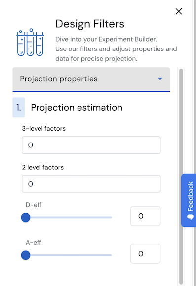
Projection properties

Often, only a limited number of the factors in an experiment turn out to have significant effects. Ideally, the design allows you to obtain a good quality second-order model involving these factors. Such a model includes all their main effects, interaction effects and, in case of 3-level factors, quadratic effects.

image info

Before doing the experiment, you don’t know exactly which of the factors will have significant effects. However, you may have some idea about the maximum number of factors involved.

In general, if you have $p$ factors and believe that at most $q$ of them can show significant effects, there are $\binom{p}{q}$ projections, and a design that performs well on average over all the $q$-factor projections is preferred.
Example: suppose that your design includes 10 factors, and you believe that at most 5 of them can show significant effects. The design has $\binom{10}{5}=252$ different subsets of 5 factors. In other words, there are 252 different projections of the design into 5 factors. A design with good average estimation quality over all 252 projections would serve your turn.

This tab allows you to specify:

The maximum number of factors that you believe to have significant effects
- The controls allow specification for the maximum number in models with only three-level factors, in models with only two-level factors and in models with a combination of three-level and two-level factors.
The minimum values for two criteria to quantify how efficiently the design quantifies a second-order model with this number of factors.
- Both the sliders and the fill-out boxes allow you to specify minimum values for the average D-efficiency, the average A-efficiency, or both.
- Both of these criteria address the statistical uncertainty in the model coefficients. This uncertainty can be expressed as the variance of the individual coefficients and the correlation of pairs of coefficients. The variance of a coefficient measures how precise the coefficient itself is estimated. The correlation among two coefficients measures the amount of cross-talk between them. If two coefficients are highly correlated, you cannot be sure which of the corresponding effects contributes to either coefficient. If they are uncorrelated, the interpretation of the coefficients is unambiguous.
- Technical considerations (click to unfold)
  - A design’s D-efficiency for a particular model addresses the variance of the model coefficients as well as the correlation between these coefficients. Maximizing the D-efficiency simultaneously minimizes the uncertainty in the coefficients themselves and the cross-talk between coefficients.
  - The A-efficiency of a design for a particular model solely addresses the variance of the model coefficients. Maximizing the A-efficiency minimizes the uncertainty in the coefficients, but leaves the amount of cross-talk between coefficients unaddressed.
  - Both kinds of efficiency can attain values between 0% and 100%. An average of 0% means that the model cannot be calculated for any of the projections. An average of 100% means that the models for the projections all have the best possible efficiency for all the projections. If the average is in between, the models don’t all have the best efficiency but neither do they all have the worst possible efficiency.
  - The technical definition of the D-efficiency of a model with p parameters (including intercept) based on a design with N runs is $$D = 100 \cdot \frac{|\mathbf{X}^T\mathbf{X}|^{1/p}}{N}, $$
    where |.| denotes the determinant, and $\mathbf{X}$ is an $N \times p$ model matrix with intercept, and further independent variables corresponding to some or all main effects, interaction effects and quadratic effects. Each effect in the matrix is normalized to a length of $\sqrt{N}$.
  - The technical definition of the A-efficiency of a model with p parameters based on a design with N runs is $$A = 100 \cdot \frac{p}{N \cdot tr[(\mathbf{X}^T\mathbf{X})^{-1}]},$$ where $tr[.]$ denotes the trace of a matrix, $(.)^{-1}$ denotes the inverse of a matrix and $\mathbf{X}$ is defined above.

The two sets of controls allow you to specify projection estimability requirements for two types of subsets of effects at the same time.